GeneNetwork: A tour and tutorial 
This text is taken from the GeneNetwork Tour available at http://gn1.genenetwork.org/tutorial/WebQTLTour. See the Help menu in GeneNetwork menu for the most current version of the Tour. You can also download a somewhat related Primer on using GeneNetwork (Williams RW and Mulligan MK, Genetic and Molecular Network Analysis of Behavior, Int Rev Neurobiol., 2012, 104: 135-157).
Aim of this tutorial.
The goal is to illustrate how to use GeneNetwork (GN) to study gene function and relations between genes and traits such as differences in disease severity, differences in anatomy, and differences in physiology and behavior. You can also use GN to study relations among phenotypes, for example: to what degree does an injection with cocaine or alcohol lead to an increase in movements? Most of the experimental data sets in GN are from small populations of mice (e.g., the BXD family of strains) and rats (HXB family). There are also some human, monkey, drosophila, and plant data sets to explore, although you may find that mapping functions have not yet been implemented for these other species.
The focus in this tutorial is how to use some of the most important functions. You should be able to complete this tutorial in about an hour. For this demonstration we will study expression of a key gene known as NR2B or Grin2b. This gene/mRNA/protein is crucial in learning and memory. Once you have worked through this example, you should be able to use GN to explore single genes or set of genes, mRNAs, and other standard traits that interest you.
What you will learn. If you spend an hour working through this tutorial you will learn how to extract dozen of molecules that potentially interact with NR2B. It will be easy for you to generalize what you learn to any other gene or transcript of interest. You should be able to confirm known relations (information from the literature) and you should be able to uncover intriguing new relations among sets of molecules and other traits. You will learn how to exploit a gene ontology (a gene ontology is a simple and systematic way of categorizing the functions of genes) and you will also learn about gene or QTL mapping and complex trait analysis.
By the way: if a term is new to you (What is a QTL?), and you would like to read a short explanation then look at the Glossary.
Much of the data in GN were generated as part of transcriptome studies (microarrays and now RNA-seq). As you have undoubtedly heard or experienced yourself, the analysis of transcriptome data sets is difficult and sometimes messy. You may encounter poor quality data in some of these enormous data sets. An important part of learning how to use GN involves tools to evaluate their quality. Treat data and results you generate with caution and skeptism. There are solutions to some problems you run into, but we do not have solutions for all problems. One of the first approaches to validating and double-checking a finding is to see whether you can replicate it in another related data set. When possible make comparisons across multiple data sets and multiple families, groups, or species. But in many cases the only good solution--if you are writing a paper based on key GeneNetwork data may be independent validation. Over the next few years we will be adding more and more RNA-seq data, proteomic data, and metabolomic data. Check for new data. They may help.
After you have worked through with this tour, please look quickly at the Frequently Asked Questions and the Glossary. Let me know if you have other questions or if you see mistakes that I should fix. Email should go to Rob Williams (rwilliams@uthsc.edu).
Step 1: Getting the terminology right.
The use of gene symbols and names in research papers is not consistent. When you search databases it helps to use the preferred or official gene name and symbol. In most papers, the NMDA 2B receptor is abbreviated NR2B and a Google search for "NR2B" will generate about 250,000 hits, many of which deal with the genetics and molecular biology of learning and memory. But it turns out that NR2B is not the official name of either the gene or protein. A great way to verify nomenclature is to go to NCBI Entrez Gene and enter the gene name or symbol. Entrez Gene should be able to resolve your query and give you the correct symbol.
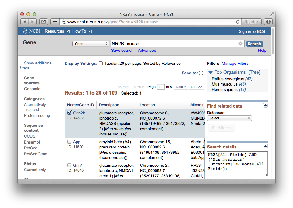
Figure 1: Getting the terminology right
When we enter NR2B or nr2b along with the term "mouse" we find that the official gene symbol in Entrez Gene in this species is Grin2b. If you search for "nr2b human" you will find that the corresponding human gene symbol is the same, but written entirely in capital letters: GRIN2B. In both species the official gene name (the description field in Figure 1) is glutamate receptor, ionotropic, N-methyl D-aspartate 2B (epsilon 2).
Step 2. Linking to the GeneNetwork search page
Now you are ready to link to the GN search page at gn1.genenetwork.org/. Ideally, keep this tutorial page open at the same time so that you can look back and forth between the two windows. You have a few choices to make: Choose Species = Mouse, Group = BXD, Type = Hippocampus mRNA. We have a great deal of gene expression and other phenotype data for the BXD family of mice, so when in doubt, select this group. Having made these three choices, you still need to pick a particular database; in this case an array data set for a particular brain region called the hippocampus that, like NR2B, is critical in learning and memory. For the purpose of this tutorial, choose the Data Set called Hippocampus Consortium M430v2 BXD (Jun06) PDNN.
You can set your particular choice of species, group, type, and database as your current default setting. Simply click on the big blue button labeled Set to Default. If you want to know what this long data set name (Hippocampus Consortium M430v2 BXD (Jun06) PDNN) is all about, click on the INFO button immediately to the right of the data set name.
Now enter your search terms into the search term field labeled Get Any or Combined. Get Any is usually best and will search for all of the entries you put in this field (logical OR). You can put at least 50 gene symbols in this field, and you can just paste them from a text file or Excel column or row. The Combined search field will only find those records that match all of the terms that you enter (logical AND). You could enter both NR2B and Grin2b in the Get Any field. You can also use wildcard characters ? and * for single or multiple characters. It is often a good idea to enter an asterisk after a search term, such as Grin*. This will get all subunits of a molecule or complex.
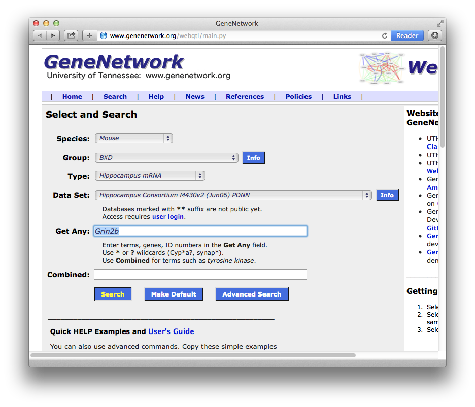
Figure 2: The Select and Search Page
Just below the Search button, there is a set of eight Quick HELP Examples of slightly more clever formats you can use to find interesting genes, mRNAs, proteins, or classical traits such as brain weight or data on learning and memory performance in mice. For example, the search string "GO:0045202" will find all synapse-associated genes currently listed in the Gene Ontology. You cannot use all of these special search commands in all data sets, but they will work for almost any Type that includes the label ...mRNA. In this case our Type is Hippocampus mRNA and any of these Quick Help examples will work.
One of the hardest parts of using GN well is knowing where to look for the right types of data. We are now trying to improve search for data in GN but we receive so much data that there are always new problems. Here are some simple suggestions:
- If you are interested in a particular species, tissue or cell type, and a gene or protein, then search as described above. GN has good coverage for mouse (particularly the BXD group), moderate coverage for human and rat, and very sparse coverage for six other species. For a general surgery of gene expression in humans, use the NIH Genotypes Tissue Expression Project (GTEx) data sets. We have entered GTEx RNA-seq data for about 40 tissue types.
- If you are interested in classic phenotypes such as blood pressure or body weight or behavioral traits, then you should start with the BXD Group and Type = Phenotypes
- If you are interested in protein expression data, then stay tuned. We will have our first quantitative data sets for mouse liver in 2014 and 2015.
- Metabolites, metagenomic data: Very sparse at present.
- Epigenetic data: Very sparse at present
- We love to answer questions by email, so do not hesitate to ask us (rwilliams@uthsc.edu).
Step 3. Retrieving the data. When you click on the Search button, your computer sends one or more string of search terms to GN, which then looks through tens of thousands of records for matching terms. The data set that we just searched has 45,101 entries that represent close to 20,000 known genes. Although some data sets include as many as 1,200,000 records (e.g., the UMUTAffy Hippocampus Exon (Feb09) RMA data set), the search results should displayed within a few seconds, provided that there were no more than 5000 hits. If there are more than 5000 records you will need to refine your search a bit. If you want to determine the total size of any database enter a single asterisk (*) in the Get Any field.
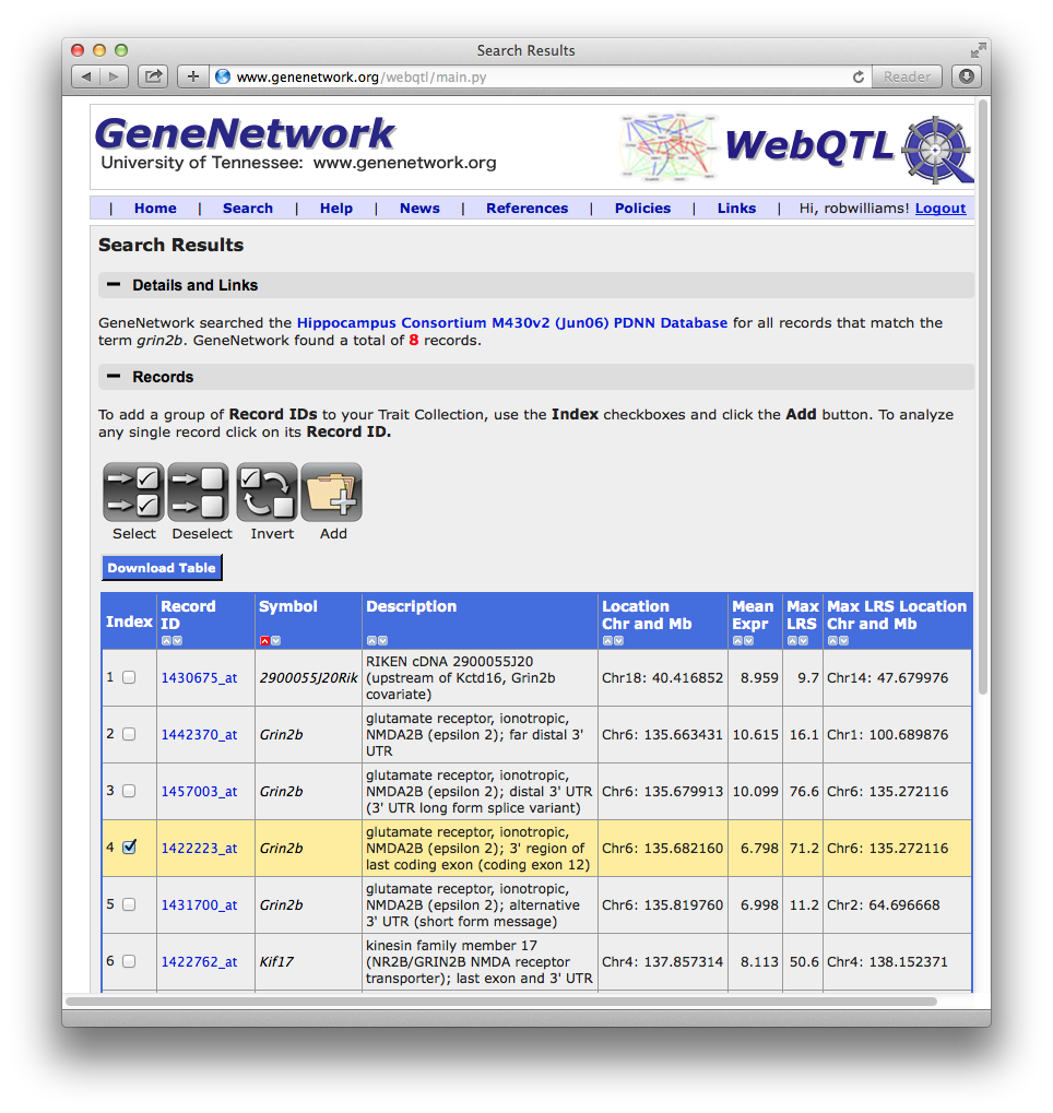
Figure 3: Search results for the search string Grin2b
In this particular case, if you enter "Grin2b" you will get at a list of eight data sets or Record IDs. Four of these (index numbers 2 through 5) are measurements of Grin2b expression. All four are measurements of mRNA levels that target different parts of the mRNA molecule: 1. the far distal 3' untranslated region (UTR), 2. the distal 3' UTR of a long-form variant, 3. the 3' region of the last coding exon (coding exon 12), and 4. an alternative 3' UTR (a short form of the message). Which of the three should you pick? The best choice is usually the one which corresponds to coding sequence--in this case the highlighted Record ID 142223_at (index number 4). You can come back to the other data sets later to see how they compare. And you can ignore all of the other rows of data that were found only because the gene descriptions happen to include the text "Grin2b"

This is a good point to stop and to review several of the features of most GN pages. Feature 1 is the banner of terms toward the top labeled Home, Search, Help, News, etc. etc. Most of these headings have pop-down lists from which you can select additional resources and tools. For example, the Search menu heading lists the Search Databases page (our starting point), the SNP Browser tool, the GeneWiki resource, Interval Analyst, and GenomeGraph displays. These features are worth trying out later. The Policies menu explains how to contact the data providers and how to use and cite data. Send us an email is you have questions about use, but in general a citation is what we hope for.
Another useful feature of the Search Results window is the sorting row at the top that contains very small arrowheads pointing up and down. You can sort the search results by symbol, description, gene location, expression levels, or by maximum LRS or LOD scores. There are also small index check boxes to the left of each entry. These are used to select data you would like to move into a Collection. The Add button will move any checked items into your collection. Collections can include any gene, trait, or SNP marker that has been measured in the BXD family. You can even add your own BXD data using Enter Trait Data in the Home menu (top left). The ability to add diverse data types into a Collection provides a great deal of power. The use of the Collections is a topic for a more advanced tour. Let's get through this quick tour and then feel free to build up your own collection of phenotypes for network analysis.
Step 4. Reviewing the NR2B expression data.
Select the checkbox to the left of Record ID 1422223_at in the Search Results window. This weird Record ID is the name that Affymetrix Inc has given to one of the specific assays of mRNA expression of Grin2b. The call their assays "probe set", and this probe set targets the last exon of the Grin2b transcript. The row will be highlighted in pale yellow. Click on the blue text "1422223_at". This will generate a new page called the Trait Data and Analysis Form.
This Trait Data and Analysis Form page is the most important page for the analysis of transcripts and other types of traits. We will return here several times. The top of this page contains useful background information, including the database that we used, the mRNA or trait identifier, gene symbol and aliases, the chromosomal location and megabase position (Mb) of Grin2b in the mouse genome. GN also includes links to NCBI, OMIM, GenBank, BioGPS, STRING, PANTHER, Gemma, and the Allen Brain Atlas (ABA). To find out more about these resource, just click on the links. There are also many additional useful links under the Links menu heading.
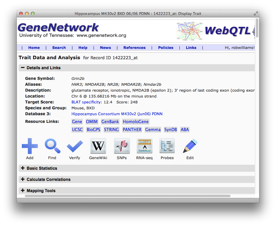
Figure 4: Trait Data and Analysis Form for Grin2b, probe set 1422223_at
Seven (or eight) large square buttons are shown in Figure 4 and you need to know what most of them do.
- Add: Use this big + button to add any trait to your collection (same as in the Search Results page).
- Find: This will find the term GRIN2B or Grin2b in many other databases (probably way more information than you want at this point, but try it anyway).
- Verify: This button is used to confirm that the probe or probe set really and truly targets the last exon of Grin2b. Click on the button. The probe sequences used on the array (or in some cases now the RNA-seq sequence) are sent to the Genome Browser and the best match is found in real time using the BLAT algorithm. The Search Results page allows you to drill down to a view of the genome. Click on the upper-most of the "browser" links to the far left (top row). Look for the horizontal track that is made up of a series of black rectangles labeled "Your Sequence from Blat Search" or "Probe 1422223_at". You will also see several horizontal "tracks" labeled Grin2b and GRIN2B. If you use the zoom out 10X button you will see that the probes and probe set are aligned with the 3' end of the last exon--a bit more detail than we had before. You may also notice that Grin2b is encoded on the minus strand of chromosome 6 and that the tiny arrowheads visible on the last intron point to the left (the transcription direction is from right to left). The RNA seq button has the same function, but takes you to a GN mirror of the UCSC Browser into which we have added RNA-seq data for brain, hippocampus, and eye (Jan 2011) of BXD strains of mice.
- GeneWiki: This link lets you annotated our databases. You can leave yourself notes and comments about particular genes or probe sets. You can easily find your own notes using a special search string described in the Advanced Search page. But in short your search would be written out "wiki=myName". Leave out the quotes and make sure that "myName" is in your Wiki entry. It is that simple.
- SNPs: This link provides you with a list of all known SNPs in Grin2b that are in the GN database. You can, of course, also search for SNPs in other genes or regions. The SNP Variant database is pretty well populated (about 60 million SNPs) and includes many SNPs from Sanger and our own in-house sequencing projects. As of April 2014, there are nearly 51,858 SNPs in Grin2b, but only 21 of these are non-redundant SNPs in eons between the two strains that concern us most here (C57BL/6J and DBA/2J). Click on the SNP Browser button to have a quick look. You may need to restrict the SNP search to just Domain = Exon, and also click on the "Non-redundant SNPs Only" box and the "Different Alleles Only" box. You will also need to Cut all strains except C57BL/6J and DBA/2J.
- RNA-seq: This works the same way as Verify, but takes you to a GN mirror of the UCSC Browser into which we have added RNA sequencing data for brain, hippocampus, and eye of BXD strains of mice. Useful if you are a neuroscientist.
- Probes: A link to the sequence data for the individual probes that make up an Affymetrix probe set. This table can be used for a very fine-grained analysis of particular probe sets, but is actually rarely used at this point.
- Edit: The Edit function appears only if you are logged into GN (upper right of all pages). Once you are logged in you can actually modify the annotations.
In general, text that uses a blue font is also a link. For example, the text at the top of Figure 4 Hippocampus Consortium M430v2 BXD (Jun06) PDNN will link you to a Materials and Methods "metadata" or Info page. There is lots of information on the Info page, but the short summary is that the NR2B expression data in the Hippocampus mRNA database we are exploring was generated from approximately 1200 hippocampii and 600 mice belonging to 99 strains (typically three animals per array and approximately 200 arrays). This is one of the largest data sets in GN. Each array includes samples from a single age, sex, and litter. The BXD strain family were all made by crossing two parental strains, C57BL/6J and DBA/2J. Both of these parents have been fully sequenced. The Hippocampus data set includes expression estimates for both parental strain, and also data for 15 other common inbred strains, for example, 129S1/SvImJ, C3H/HeJ, CAST/EiJ, and others. There is also a complementary, but smaller Hippocampus Consortium data set for the CXB strains of mice.
Farther down the page we encounter four grey horizontal bands labeled Basic Statistics, Calculate Correlations, Mapping Tools, andReview and Edit Data. We will come back to these tool areas in a moment, but keep scrolling down to look at the actual numerical data on gene expression for Grin2b.
The larger numbers in the boxes (6.722, 6.695, etc.) are estimates of the abundance of Grin2b mRNA in the hippocampii of different samples of mice. The smaller numbers (0.308, 0.383, etc.) are the standard errors of expression, usually based on two arrays (because n = 2 the SEM also equals SD). Numbers are all expressed using a log base 2 scale. A value of 8 therefore corresponds to 2^8 or 256 on a linear scale. A difference of one unit is roughly equivalent to a two-fold difference in expression in Grin2b expression. B6D2F1 at the top has an expression of 6.722 +/- 0.308 whereas BXD45 has an expression of 7.790 +/- 0.076. That amounts to approximately a 2-fold difference in the amount of transcript.
These kinds of preliminary results often generate intriguing and testable hypothesis: do strains of mice have the anticipated differences in learning and memory performance given the known effects of Grin2b overexpression in transgenic mice? If you scroll down farther in this lists of Grin2b expression estimates you will see that the strain of mouse called BXD73a (once known as BXD80) only expresses 6.154 units of NR2B whereas BXD42 expresses 8.557 units. That amouts to a putative 5.29-fold difference in mRNA level. We need to take this with a grain of salt, because these estimates are lower than we expect. The average expression for all transcripts (including those NOT expressed) is 8 units. The fact that the average expression of this Grin2b probe set is less than average should make us worry. Are these data too noisy to use? Is there an unsuspected problem with the data handling or the Affymetrix probe set? These are hard questions to answer but the Probes tool is useful because you can look at the expression of the individual probes values that are used to generate the probe set summary. We will skip this process for now, but remember that this "deeper" level is just one click away. For the time being, let's evaluate the data using the Basic Statistics functions.
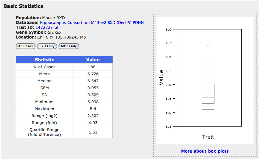
Figure 5: Basic statistics for Grin2b
Step 5. Basic Statistics. To get a better understanding of these values and how expression estimates are distributed click on the Basic Statistics button. A new window will open with a statistical summary table and a box plot toward the top (Figure 5), two bar charts in the middle, and a normal probability plot toward the bottom. You may not be familiar with these types of plots yet, but they are simple to read. The box plot is a simply summary of the spread of the 86 values. The blue plus sign represents the mean expression. The box defines the 25% and 75% quantiles (if we had studied exactly 100 strains these would be those strains at the 25 and 75 rank. If you want more information, just click on the link beneath the plot.
The bar charts are easy to read. They provide a graphic output of the data that you saw in the Trait Data and Analysis Form. The Y axis of the graph is truncated and does not extend down to a value of zero. This tend to highlight the variation within strains. The error bars are quite large, and are only based on two samples (in this case the SEM is usually the same as the SD). Also note that the size of these error bars tend to increase as the expression increases (non-uniform error). High noise and non-uniform variance are all characteristics that should reduce your enthusiasm. But let's persevere, because these data have not yet cost you a penny and because this is a great lesson.
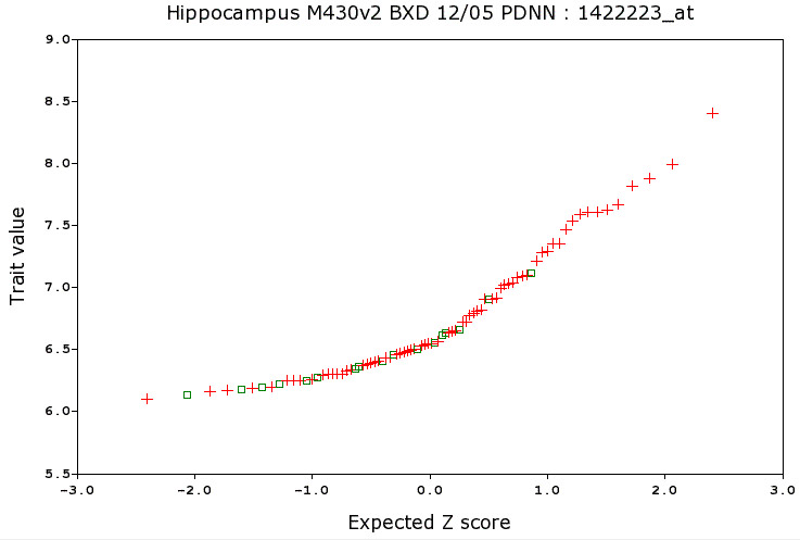
Figure 6: Normal Probability plot for Grin2b
Toward the bottom of the Basic Statistics page you will find a Normal Probability plot (Figure 6). There is another link associated with this plot that will provide more background, but here is a brief explanation of how to read these plots. On the X axis is the expected Z score for every strain based on its ranking out of 86 strains. Values range from about -2.5 to +2.5. If you randomly drew 86 values from a normal distribution you would expect the lowest value to be about -2.5 standard deviations below the mean (or -2.5 Z) from the mean. The Y axis provides a read-out of the actual expression level. If the expression of NR2B were normally distributed then the strain averages would form a straight line. If expression of Grin2b were obviously controlled by a single Mendelian factor, then this plot would have an S shape with many high strains and many low strains and few strains with intermediate values. Instead this plot highlights skew toward low values (also seen in the box plot). A few strains have comparatively high expression, but the main feature is the excess of strains with values from 6.0 to 6.5 units. It does not look like a Mendelian trait. But looks can deceive.
What this plot also highlights is the wide range of expression of NR2B gene transcript in normal strains (the BXD strains are not mutant or knockout mice). But the high error raises the possibility that much of this variation is simply sampling error. If we performed an analysis of variance with Strain as our main effect, this data set would be associated with a modest and statistically insignificant F values. But we have other methods to evaluate this putative strain difference. We can map it and see if any interesting patterns emerge from the mapping that might cheer us up and demonstrate that the variation of strain means is actually true signal. In this case, the answer is (fortunately) a strong Yes (LOD = 16). But when you see data of this type, the usual answer will be No.
Variation in NR2B gene expression is a signal that we can now cautiously use to search for transcripts that co-vary. Does NR2B message covary with other subunits of the NMDA receptor complex (over 1000 transcripts are part of the postsynpatic density of which NR2B is a key member). Does the the expression of other genes compensate for the apparent 5-fold range in NR2B message level?
Step 6. Covariation of expression. To answer these types of questions return to the Trait Data and Analysis Form that has all of the values for Grin2b in 86 different strains of mice. This time select the Trait Correlation button. There are five pop-down menus that allow you to modify search parameters.
Let's modify one of the default settings. Change Return to read top 500. The other seetings are fine for the time being. Now click on the Trait Correlations button.
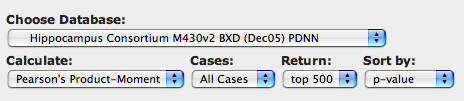
Figure 7: How to set up the search for covariates of Grin2b
Within a few seconds of clicking this button, GN will return a new page of data, a Correlation Table of the top 499 transcripts that covary with variation in Grin2b expression. At the top of this list (sorted by p value) is Grin2b itself. The third best covariate of our Grin2b probe set is another Grin2b probe set. That is reassuring.
Let's review the columns:
- The first column is just an index with check boxes. You can easily add items into your BXD Collection using these checkboxes.
- Record ID: The ID of the trait; in this case just the probe set identifier given by Affymetrix
- Symbol: The official gene symbol. Clicking on these symbols will link you to NCBI.
- Description: The name of the trait or the name of the gene from which the mRNA is transcribed
- Chr: The chromosome of the gene from which the transcript is transcribed
- Megabase: The chromosomal nucleotide position of the most proximal end of the probe set (mm6 alignment)
- Mean Expression: The average expression of the probe set (mean of strain averages)
- Correlation: The correlation of with the reference trait, in this case with Grin2b probe set 1422223_at.
- N Cases: The number of strains involved in the correlation analysis
- p Value: The p value associated with the correlation and number of cases without correction for multiple tests.
- Lit Corr: The Literature Correlation. This is a very cool column of data generated by Ramin Homayouni, Michael Berry and colleagues that summarizes the correlation of Grin2b with many other genes based upon an analysis of the PubMed Literature.
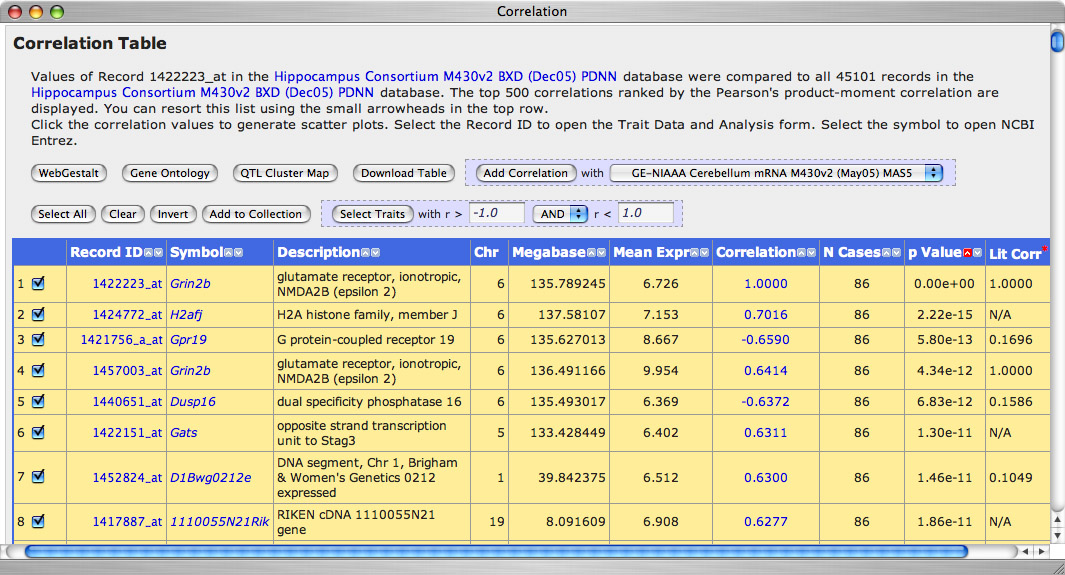
Figure 8: Correlation Table
Clicking on any correlation value will generate a scattergram ofGrin2b on the X axis and the other transcript on the Y axis. For example, the scattergram of Grin2B (X axis) versus Grin2b is shown in Figure 9. The p value associated with this correlation is highly signficant and is listed in the upper right corner for both the parametric Pearson's r value and for Spearman's rank order r value. GN generates the Correlation Table after performing 45,100 statistical tests; so we should correct for multiple tests. In this case, the p value is significant even if we apply a stringent Bonferroni correction. You may regard this Grin2b-to-Grin2b correlation as somewhat of a disappointment, but the more you appreciate the great complexity of mRNA metabolism, the less suprised you will be. If you were planning follow-up functional or behavioral studies of strains with high and low Grin2b expression you would obviously want to resolve some of the discrepancies at the protein level or you could (with some risk) just select strains with high or low expression for all forms of Grin2b (BXD15, BXD24, BXD60 vs BXD14, BXD42, BXD96).
Correlation Tables can be resorted. Click on the the small arrowheads in the header column to resort by the Literature Correlation. You will find that Grin2b actually does covary reasonably well with Grin1 (r = 0.501). Generate the scatter plot for Grin1 and Grin2b.
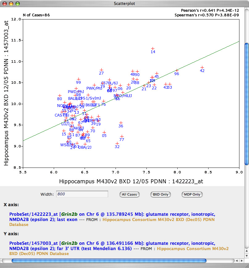
Figure 9: Scatter plot of two probe sets that measure expression of different parts of Grin2b.
Step 7. Gene ontology analysis. At the top of the Correlation Table is a button labeled Gene Ontology. When you click on this button GN sends a list of gene IDs to the WebGestalt server for analysis. Before you click on this button you need to decide which list of transcripts to send to WebGestalt. The easy answer is to send all 500 transcripts. To do this click on the Select ALL button. This action will highlight all 500 transcripts. Now click on the Gene Ontology button. The output will be a large graph consisting of three major categories and a "bush" of subcategories.
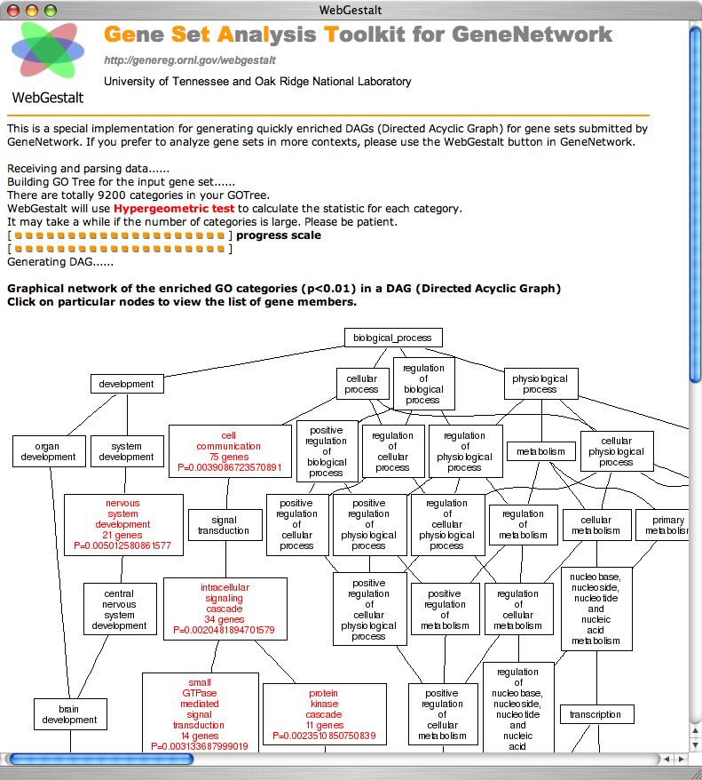
Figure 10: Gene ontology analysis with WebGestalt
A gene ontology is a hierarchical categorization of genes by their functions. A large subset of the roughly 20000 genes measured using microarrays have been assigned to one or more functional categories. The three independent trunks of this ontology are "biological process", "molecular function", and "cellular component". Within each of the the GO category we see the number of genes included in this category and the p value. For example, for the category "Nervous System Development, the numbers are 21 genes with a p value of 0.005. You can click on the category and generate the list of all 21 genes--from Acsl6 (the only covariate with a negative correlation) to Ulk1. The single category that has the highest "enrichment" is the molecular function "binding" with a p value of about 0.0000001. This category includes 261 of 500 transcripts on our Grin2b list.
Step 8: Mapping Grin2b. At this point we have gained some confidence in the Grin2b expression data. While the expression values are low, they seem to be correctly associated with moleculates enriched in the postsynaptic complex. What causes the variation in Grin2b expression among strains of mice? The simple but unsatisfying answer is that differences are caused by genetic variation between the parental strains that are inherited by the BXD progeny. The WebQTL module of GN can give us much better answers. WebQTL can tell us where in the genome this genetic variation is located and which parental strain (C57BL/6J or DBA/2J) is associated with higher expression. These chromosomal regions are the ultimate, but most distal (upstream) causes of variation in Grin2b mRNA levels. These sources of variance can be mapped like any other heritable trait. The method we use to do this is called complex trait analysis or quantitative trait locus (QTL) mapping (hence the term WebQTL). The method is covered at an accessible level in a previous SfN Short Course article.
But now we will skip the details and proceed directly to the results. Go back to the Trait Data and Analysis Form and click on the Interval Mapping button.
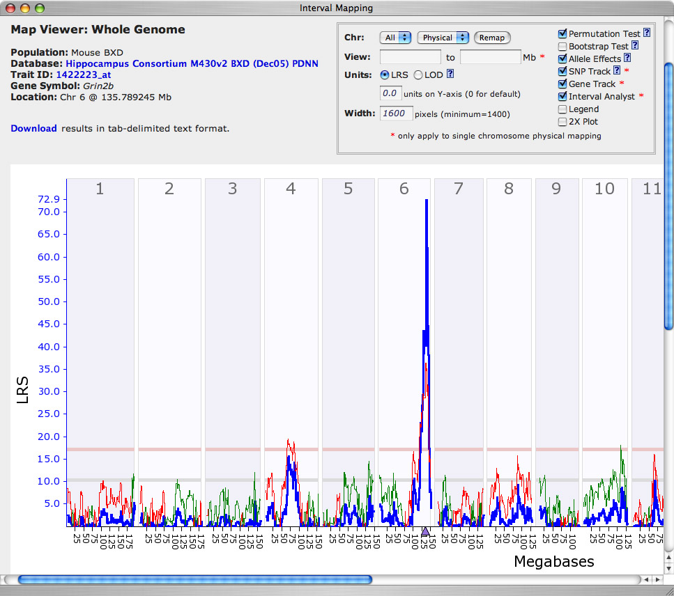
Figure 11: QTL map for Grin2b
An Interval Mapping Result window will automatically open after a short pause during which WebQTL calculates and assembles results based on 4 million linear regression equations. The window should have to a single major spike on the right side of chromosome (Chr) 6. The X-axis is a linear representation of all mouse chromosomes, as if they were tied end to end (Chr 1 to the left, and Chr X to the far right). The Y-axis and the bold lines (blue) provide estimates of the likelihood that differences in NR2B expression are modulated by polymorphic loci (allelic variants). Likelihoods are presented using a chi square statistic called the likelihood ratio statistic (LRS). Big numbers are good in the sense that they signify that we have successfully identified a chromosomal interval that controls Grin2b expression. In this case, the number is extraordinarily high, with a peak LRS of 72.9 (LOD of 15.8) on Chr 6. The horizontal gray line and the and pink line are the statistical thresholds. If the spikes exceed the upper rose-colored line, then the linkage between the chromosomal interval and variation in Grin2b expression is significant. In this case, only the Chr 6 linkage is significant, whereas that on Chr 4 at about 70 Mb is suggestive.
Step 9. Evaluation of candidate genes. Note that on the X-axis just under the largest spike there is a small purple triangle. This triangle indicates that genetic location of the Grin2b gene itself. The correspondence of the QTL and the location of the Grin2b gene suggest that polymorphisms in Grin2b modulate expression (for example, a variant in the Grin2b promoter). The finer jagged line (red or green) provides a gauge of whether DBA/2J (green) alleles or C57BL/6J (red) alleles contribute to higher expression of Grin2. See the far right axis to see how to read this "additive effect" scale. In this case, the allele or haplotype inherited from C57BL/J (red line) contributes to higher expression of Grin2b. Just to make sure, let's zoom in on the map of Chr 6 and confirm that the QTL does align with Grin2b. To zoom the map, click on the chromosome number (Chr 6) in the whole-genome interval map. This will generate a chromosome 6-specific map of Grin2b expression. Once you have this Chr 6 map on your screen, you can zoom again by clicking on the rose-colored horizontal bar at the top of the map. You will end up with a map that looks somewhat like Figure 11, in which the strongest position candidate is obviously Grin2b itself. We have informally "cloned" a QTL for Grin2b expresssion.
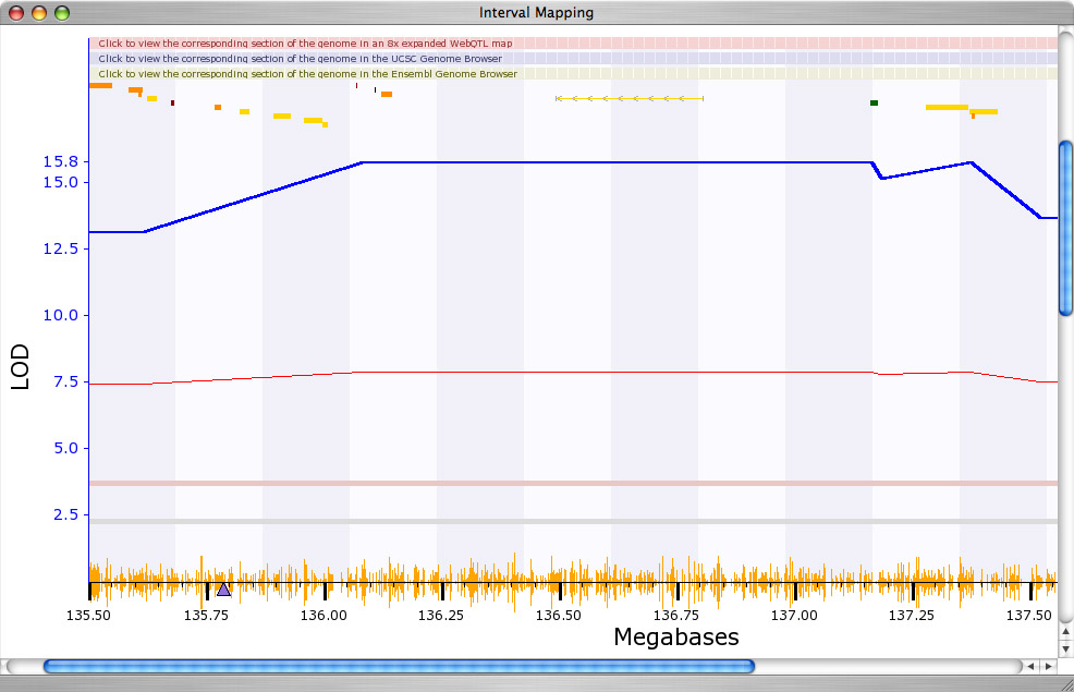
Figure 12: Zoomed QTL map for Grin2b on Chr 6
Having mapped the major controller of Grin2b expression, we can ask if any of the "left-over" variance can be explained by secondary QTLs. We can use either Composite Interval Mapping or the Pair Scan mapping function (to gain access to Composite Interval mapping you first need to click on the Marker Regression button). Both of these mapping methods are somewhat more advanced than simple interval mapping. Without going into the details (the data are weak), there is a hint that a region near the centromere of Chr 2 may also affect Grin2b expression by interacting non-additively with the Chr 6 variant of Grin2b.
Conclusion. The tour you have just taken has led your through typical steps in analyzing and evaluating gene expression data. This tour may also have generated a number of intriguing hypotheses about the relations of NR2B to itself and with molecules in the hippocampus. You can repeat this type of analysis with any of about 20000 other genes in this data set. You can do the same analysis for complex sets of transcript and traits. you can also repeat this type of analysis in other tissues. It takes time, but the cost-benefit ratio is high.
Step 10. A simple self-test
Question1. Can you verify any of these NR2B results using a different data set such as the SJUT Cerebellum M430 data set? What does a success or failure indicate?
Q2. Are there any functionally interesting correlations between Grin2b expression and behavioral traits in these same strains of mice? (Hint: generate a Correlation Table of Grin2b with traits in the Published Phenotypes database.) What is the importance of a correlation and what mechanisms can generated these correlations? Can very high correlations still be entirely spurious?
Q3. Do NR1 (Grin1) and NR2B (Grin2b) share common modulators on Chr 8?
Caveat emptor: Always be skeptical regarding results. There are pitfalls of this type of analysis highlighted in some of the questions above. These are more than counterbalanced by tremendous opportunities. Consider GN as a great tool to generate interesting new hypotheses, and be prepared to validate or refute these hypotheses using independent data and direct experimental tests.
--------
ANSWERS: Q1. No, verification is not possible using the Cerebellum data set. Different tissues have different expression patterns and control.
Q2. Yes, you should get a high correlation with rearing movements after a cocaine injection (a paper by B. Jones et al., 1999). Yes, very high correlations can be "functionally" spurious and can arise from linkage disequilibrium, sampling error, or (we hope rarely) poor experimental design.
Q3. No.
This work was supported by a Human Brain Project funded jointly by the National Institute on Drug Abuse, National Institute of Mental Health, the National Institute on Alcohol Abuse and Alcoholism, and the National Science Foundation (award P20-MH 62009 and P20-DA 21131 to KFM and RW) and by a separate grant from The National Institute on Alcohol Abuse and Alcoholism (INIA grants U01AA13499, U24AA13513 to RW).
(Text version of March 4, 2016 by RW
|