|
Frequently Asked Questions

Questions
- How do I report an error or program bug?
- Expression levels are often measured by several probes or probe sets. Which is better and which should I use?
- There are often mutliple database. Which database is best?
- How should we cite the GeneNetwork and WebQTL, and what are conditions on use of data?
- How can I compare the correlates from two transcripts that interest me? Let's say I am interested in transcripts that correlate well with both Drd1a and Drd2.
- If I have a list of transcripts that covary with Drd1a how to I decide if the correlations are truly significant or informative?
- How much would it cost to add transcriptome data for an organ, tissue, or cell type that is more relevant for my research?
- How many genes and transcripts are in the expression databases, and what fraction of the genome is being surveyed?
- The Correlation Results window includes a maximum of 500 traits. How can I generate a complete list of all correlations?
- Validation: Are there great examples of validated QTLs and correlation results? What is the proof that relations detected using GeneNetwork are biologically compelling and meaningful?
- Relevance to protein expression: Are measurements of steady-state mRNA levels relevant? Cells operate principally in the proteome domain, and there are many examples of poor correlations between mRNA and protein levels.
- What is the best way to handle a whole set of interesting traits or transcripts simultaneously? For example, can I study the genetics of all dopamine receptors simultaneously?
- What web browser do you recommend?
- Reverse mapping: How can I find a set of transcripts and other traits that are possibly controlled by a transcription factor or other gene variant that I already know about? For example, in the paper by Chesler et al., the region near D6Mit150 is nominated as a master controller. What are some of the controlled traits? How to I review them efficiently since they are not all listed in the paper?
- Finding transcripts that modulate their own expression levels (cis-QTs and cis-QTLs): How can I find a set of transcripts or proteins that are under tight control by a locus that overlaps their own physical location in the genome—that have a cis-QTL? This class of transcripts is particulary interesting because polymorphic genes that modulate their own expression, may also produce numerous downstream effects.
- How do you error-check data?
- Is there a way for me to automatically generate a log file of my use of the GeneNetwork and WebQTL?
- How can I determine the precise region of the transcript that is targeted by a particular Affymetrix or Agilent probe set?
- What expression levels are considered high and reliable; what expression levels are so low as to disregard?
- How do I select the best strains to study to improve the precision of my current mapping/QTL results?
- How do I output the genotype data associated with a particular data set? For example, I want the genotypes used in mapping BXD data.
- I have generated some phenotype data that I would like to put into GeneNetwork. How should I name my traits?
- How do I combined mapping data from two or more crosses to end up with a cumulative or summary LRS or LOD QTL map?
- How can I find a set of transcripts or proteins that have a cis-QTL or cis eQTL?
- Partial Correlation: What is it and how do I use it?
Answers
Q1: How do I report an error or program bug?
A1: Software errors that generate on-screen error messages are automatically logged and reviewed by us, usually on a daily basis. If you note an error on the public site (rather than the less stable beta site) that is persistent (more than one day) or that is really causing you trouble, please send us an email notification immediately and we wil do our best to resolve the problem. Email us at:
rwilliams at uthsc dot edu, lyan6 at uthsc dot edu, zachary.a.sloan at gmail dot com, acenteno at uthsc dot edu
[RWW, November 17, 2017]
Back to Index
Q2: Expression levels of some transcripts are measured by two or more probes or probe sets, but these values do not correlate well with each other. For example, two probe sets that target Bcl2l have no correlation with each other, whereas two probe sets for Erbb3 show a strong negative correlation (r = -0.74 using the UTHSC Brain mRNA U74Av2 RMA data set). In cases such as these which probe set should I trust?
A2: Probes vary greatly in hybridization properties and sensitivity to cross-hybridization. They also target different exons and different parts of the 3' untranslated regions of transcripts (3' UTR). A very small number (<0.1%) also contain SNPs that can affect hybridization efficiency.
The quickest answer is to use the set of probes with the highest and most consistent expression. Higher intensity signals usually have a higher signal-to-noise ratio. Select the Probe Information page from the Trait Data and Analysis form. It is interesting (and sometimes scary) to compare the mean and standard error of the mean (SEM) of the signal of different probes in the set. Also check the heritability estimate of the entire probe set in the Basic Statistics page. Heritability is a often a reasonably good indicator. You can also compare the lists of top 100 correlated transcripts for the different probe sets and see if one probe set makes more sense given the known biology and function of the gene.
There are other important features that you may want to examine.
- Check the placement of the probes that are part of the probe set. Use the Verify UCSC or Verify ENSEMBL button next to the probe set position in the Trait Data and
Analysis window. The Verify functions will BLAT the concatenated probe sequences (overlap is trimmed away) to the most current mouse genome assembly. If the placement and annotation appears to be wrong, please email us.
BLAT analysis of Erbb3 reveals a relatively complex situation. The two probe sets target different Erbb3 expressed sequence tags (ESTs).
- Use the Probe Information link in the Trait Data window to view exon
targets and the original probe sequences and their mean expression.
- Select all the probes and add them to your BXD selections. Use the Custer Map
to view the probe-specific QTLs. Strong cis QTLs detected only in a group of tightly overlapping
probes may indicate a SNP.
- Each probe can be examined as an individual trait. Check the noise of the
probe using Basic Statistics window.
- Individual probe sequences can be BLATed to the genome using UCSC's BLAT
function. You can also retrieve the sequence data to compare individual probes by
location and known polymorphisms.
- Also from the selections page, use the Correlation Matrix function to generate a
correlation matrix and perform a principal component analysis (PCA). The PC scores can be used as "consensus
traits." You can eliminate probes that appear to misbehave from you selections
prior to performing the PCA. [EJ Chesler, Oct 2004; minor update by RWW, Jan 2004]
Back to Index
Q3: There are often mutliple database versions associated with each tissue or experiment. Which database is best?
A3: GeneNetwork often provides several complementary transformations of data sets, for example PDNN, RMA, and MAS5. The Position-Dependent Nearest Neighbor (PDNN) method of Zhang and colleagues generally gives better results than two more common alternatives--RMA and MAS5 transforms.
To determine the best data set among alternatives do this: enter the string "CisLRS=(50 1000 10)" into the ANY search field for the first of the alternatives that interest you. This is one of GN's Advanced Search strings that finds all transcripts that are associated with a very strong quantitative trait locus (QTL) very close to the location of the gene. The command translates as "find all transcripts with an LRS value above 50 and less than 1000 that is located within 10 Mb on either side of the gene." GeneNetwork will compute the number of transcripts that are associated with very high LRS or LOD scores. The great majority of these hits are naturally genes that modulate their own expression. This number is an excellent measurement of data quality. GN will open a new page with the total numbers of hits. The number will be listed in red font toward the top of the Search Results page. For example, there are several alternative data sets for the cerebellum of the BXD genetic reference panel. If you systematically test each of these you will get the following results:
- n = 130 GE-NIAAA Cerebellum mRNA M430v2 (May05) RMA
- n = 117 GE-NIAAA Cerebellum mRNA M430v2 (May05) MAS5
- n = 207 GE-NIAAA Cerebellum mRNA M430v2 (May05) PDNN
- n = 514 SJUT Cerebellum mRNA M430 (Mar05) RMA
- n = 732 SJUT Cerebellum mRNA M430 (Mar05) PDNN
- n = 420 SJUT Cerebellum mRNA M430 (Mar05) MAS5
- n = 91 SJUT Cerebellum mRNA M430 (Oct04) MAS5
- n = 228 SJUT Cerebellum mRNA M430 (Oct04) PDNN
- n = 130 SJUT Cerebellum mRNA M430 (Oct04) RMA
- n = 85 SJUT Cerebellum mRNA M430 (Oct03) MAS5
In this case, the 5th data set is significantly better than all of the other transforms or data sets (n = 732 trnscripts associated with LRS values above 50 (a LOD score > 10). There is really no way to systematically generate high numbers of these so-called cisQTLs as an artifact. One of the advantages of large transcriptome mapping data sets is that we have internal but entriely objective measures of data quality. The only caveat is that some of the cisQTLs will be generated by hybridization artifacts (SNPs and other sequence variants). However, this is generally an artifact of the array platform and not of the transformation method.
When available we recommend using databases that have the suffix HWT, for example the database "UTHSC Brain mRNA (Dec03) HWT1PM." The heritability weighted transform (HWT) accentuates meaningful variation in probe signal and takes advantage of the unusually large data sets used by GN. HWT outperforms PDNN for the majority of probe sets as assessed by the strong covariance among probe sets in single data sets and in terms of the yield of QTLs at a fixed false discovery rate.
Manly KF, Wang J, Williams RW (2005) Weighting by heritability for detection of quantitative trait loci with microarray estimates of gene expression. Genome Biology 6:R27 Full Text HTML and PDF Version.
MAS5 and dChip do not generally perform as well as the other transforms. However, there are a few probe sets for which MAS5's reliance on the mismatch probe actually does improve performance, one instructive example being the transcript of Pam using the selection sequence Mouse -> BXD -> Striatum. WebQTL also provides access to the primary probe signals, and it is possible to generate custom probe set consensus expression estimates by performing a principal component analysis of all or a subset of probes (see the previous question). [RWW, Dec 14, 2004; Sept 25, 2005; April 23, 2006]
Back to Index
Q4: How should we cite the GeneNetwork and what are the conditions on use of data?
A4: Please cite GeneNetwork in text using this format recommended by the Neuroscience Information Framework: GeneNetwork (date accessed), RRID:SCR_002388
Please also have a look at the References page or at the Usage Conditions page. If you have other questions about a particular data set, please link to the Contacts page or Info button for the individual data sets. [RWW, Dec 14, 2004; Feb 23, 2005; Jan23, 2018 ]
Back to Index
Q5: How can I compare the correlates from two transcripts that interest me? Let's say I am interested in transcripts that correlate well with both Drd1a and Drd2.
A5: The two traits need to have been measured using the same genetic reference population, such as the BXD strains. But it is ok if they have been measured in different tissues. Put Drd1a and Drd2 transcripts into a single Selections window. Click on their small selection boxes, and then use the Compare Correlates function. [RWW, Dec 23, 2004]
Back to Index
Q6: If I have a list of transcripts that covary with Drd1a how to I decide if the correlations are truly significant or informative?.
A6: In most databases correlations under 0.7 will have relatively high false discovery rates (FDR). However, this statement needs to be moderated if you already have strong prior data that suggests that such correlation should exist. The Literature Correlation column (far right) tries to formalize the likely biological connection between two genes based on a comparison of PubMed abstracts for the genes.
One can compute a formal FDR for the data in a correlation table given the size of the array, but the FDR does not account for the noise structure of the array data. Structured noise, such as batch effects, can seriously inflate correlations. We recommend that your biological sense of the system you are studying be a major "prior" in evaluating a list of correlations. You can also compute the Gene Ontology stats for the top 100 or 500 transcripts. A "bad" list should not generate an interesting GO structure.
Here is an operation that will help you in evaluating the significance of correlations: Search the ANY field using this string "mean=(1 5)". This will find probe sets with very low expression. For example, in the BXD Whole Brain INIA PDNN data set, this search string returns 10 probe sets. For example, the correlation table for Abcd2 (probe set 1439835_x_at_B) starts at a high value of r = 0.65. Similarly, Myo1f has a top covariate of 0.73 but then shifts down immediately to 0.64. These correlations are not likely to be biologically meaningful, particulary without strong prior data.
[RWW, May 12, 2006]
Back to Index
Q7: How much would it cost to add transcriptome data for an organ, tissue, or cell type that is more relevant for my research?
A7: Around $20,000–$40,000 for a medium-sized study; high quality arrays cost around $300-$400 each. A minimum sample size is two biological replicates for each member of the genetic reference population (GRP), often one male sample or pool of male samples, and one female sample or pool of female samples. If the GRP contains 40 genomes or strains, then you need to budget for a minimum of 90 arrays (10 for control, wastage, and reruns). Ideally all of the samples should be processed in one large batch, although batches of 20 or more arrays can usually be normalized to each other fairly well. We would be happy to help generate new data sets at any stage, the earlier the better. [RWW, Dec 23, 2004; EGW Apr 11, 2012]
Back to Index
Q8: How many genes and transcripts are in your databases, and what fraction of the genome is being surveyed?
A8: The U74Av2 data sets (brain and hematopoietic stem cells) contain ~12,400 probe sets that target about 9,000 different UniGene clusters. A UniGene cluster is a group of real and putative mRNAs that appear to be generated from a single gene (unified gene). The M430 data sets contain ~45,000 probe sets that target at least one member from each of ~32,000 nonredundant UniGene clusters out of a total of 46,000 clusters in the most recent UniGene build (#143) of Mus musculus.
What fraction of the genome and transcriptome does this represent? According to the most recent AceView summary (Nov 2004), there are 51,000 main genes (well-supported genes that code for proteins with at least 100 amino acids or that contain conventional introns) in the human genome. There are another 60,000 putative genes, some of which may be pseudogenes. Finally, there are an additional 229,000 so-called cloud genes that have a few associated GenBank sequences (usually less than 6 entries) but do not contain introns and do not code for protein (no open reading frame). These cloud genes are often intercalated in the right orientation near or in main genes. The mouse genome is likely to have nearly the same numbers of these three categories of genes. The majority of main genes are associated with multiple alternative splice variant transcripts, often more than 5. Thus, old COT curve estimates that there are 200,000 or more unique transcript species in a single tissue such as the brain are entirely plausible.
In summary, the Affymetrix M430 2.0 array is likely to represent 50% to 70% of main genes, an unknown fraction of putative and cloud genes, and a more modest fraction of the entire transcriptome. However, it is likely that the M430 array samples at least one common transcript (or a collection of transcripts with the same 3' UTR) from the great majority of abundant and widely expressed genes that have 50 or more UniGene GenBank entries. Array platforms of this type can therefore be called "whole genome" arrays without too much inaccuracy. They cannot be considered true "whole transcriptome" arrays.
The Agilent G4121A toxarray consists of 20868 60-mer probes and is likely to represent 40% of so-called main genes listed in AceView.
[RWW, Jan 1,2, 2005]
Back to Index
Q9: The Correlation Results window includes a maximum of 500 traits. How can I generate a more comprehensive list of all correlations?
A9: Select the SEARCH menu item labeled Simple Query Interface. Select the appropriate menu items, enter the trait identifier (a specific ID), and chose an output order and format. The output can be saved as a tab-delimited text file and imported into spreadsheet and statistics programs.
[RWW, Jan 2, 2005]
Back to Index
Q10: Are there strong examples of validated QTLs and correlation results? What is the proof that relations detected using GeneNetwork aare biologically compelling and meaningful?
A10: Yes, there are already several examples, and we expect the number of validated results to increase rapidly along with the depth and quality of data sets. Here are examples:
- Pumilio 2 is a mouse homolog of the Drosophila RNA-binding gene pum. The PUM protein in Drosophila binds to a 3' UTR Puf domain in a number of mRNAs and strongly inhibits their translation (a translational repressor). While the mouse pumilio homologs of this well conversed eukaryotic gene have been known for several years, there were no known mRNAs that are PUM2 targets. Using WebQTL, Scott and colleagues (2004) noted strong positive correlations between Pum2 and Rbbp6/P2P-R message levels in three transcriptome data sets (forebrain, cerebellum, and hematopoietic stem cells). P2P-R is an important nuclear gene (also known as retinoblastoma binding protein 6) that is involved in p53-mediated transcriptional control. The robust covariance between Pum2 and P2P-R suggested that P2P-R was a target of Pum2 repression. Three nearly perfect Puf domains were subsequently found in the 3' UTR of the P2P-R 3' UTR, providing additional bioinformatic support. Subsequent pull-down experiments carried out by E. White-Grindley and E. Ruley provide the final confirmation that PUM2 protein binds to P2P-R mRNA. [RWW, Jan 8, 2005]
Scott RW, White-Grindley E, Ruley HE, Chesler EJ, Williams RW (2004) P2P-R expression is genetically coregulated with components of the translation machinery and with PUM2, a translational repressor that associates with the P2P-R mRNA. Journal of Cellular Physiology, in press. Full text HTML version
- Retinoblastoma binding protein 7 (Rbbp7, Mis16 or p55, probe set 1415775*) is part of the core histone deacetylase complex that modulates nucleosome structure via effects on histone transport and acetylation, and DNA methylation. Together with RBBP4 (1434892*) and several other proteins such as BRCA1 (1424629*), MTA1 (1417295*), MBD3 (1417728*), HDAC1 (1448246*), and HDAC2 (1445684*), RBBP7 protein helps suppress levels of transcription, enhances apoptosis, and inhibits cell growth and transformation (Cheng et al., 2001). The gene maps to Chr X at approximately 153 Mb. Its expression is comparatively high in brain and kidney (Yang et al., 2002). We have shown that variation in Rbbp7 expression in the striatum of BXD strains is substantial. Expression is high in C57BL/6J and comparatively low in DBA/2J (1415775* in the HBP/Rosen Striatum M430v2 11/04 PDNN data set). This variation is caused by a strong QTL that peaks very near to the Ahr marker (LRS of 21.3; also see the adjacent marker D12Mit153) on proximal Chr 12. Ahr is not a typical marker; it is actually the aryl hydrocarbon response gene (1449045* and BXD Published Phenotype ID 10371). The AHR protein is an important transcription factor that complexes with the ARNT nuclear translocator (Affymetrix probe set 1437042*) and binds to xenobiotic response elements and AhR elements in promoters to influence gene expression. There is a critical leucine-to-proline substitution in the Ahr gene that results in a 15 to 20-fold reduction in the binding affinity of the proline variant found in DBA/2J compared to the b-1 leucine variant found in C57BL/6J (Chang et al., 1993). Furthermore, the DBA/2J sequence converts a normal opal stop codon at 36185363 nt (mm9) to an Arg residue (rs3021951) and thereby extends translation for an extra 43 amino acids. Note that Published Phenotype ID 10371 demonstrates an 80-fold variation in Ahr induction by anthracene that unequivocally maps to the Ahr gene locus on Chr 12 (despite the title of the 1984 paper by Levgraverend and colleagues). For this reason Ahr is an unusually compelling candidate gene. If variation in the binding affinity of AHR isoforms causes expression difference, then we naturally expect an AhR element in the promoter of Rbbp7. The 5' UTR and proximal promoter of Rbbp7has the following sequence:
ACACC GCGCT CGCAT CCGCC CCACC CCCGC GCGGG CCCAG CCGCC CCCGC GGCCA GCCTG GGGAG TGACG CCTCG CGCCT GCGCC TCGCC GACTT CCTGC
CGCGG AACGC CCCAC CCACT CTCGA GAAGC CCACC CCCGG AGAGC GCGTC AGACC CTCCC GTCGC ACGCT ATTGG TCCAA GCCGC CGAGC CGTTG GCTCC
CAGGC CCGCC TCTTC TCCGC CTCTC CAATT TCCCA GGGCG GCTGC GCCTG CGCTC AGCTG CCTGG GCGGG CTGAG AGGCG CGGGT TGAAA AGTCT CGTTC
CAAGT TTGGC GAGAG GGAGA GAGAG GAGAG CGGCT CAGAC CTCGC TACCC GCCAG CGGGG AGGAG GCAG AAGAG GAGAT CGCGG CGTCT GGGGG GAGAA
CCCAG ACGGC CAGAC CGAAC TCAGG CTTTT CCGAG CGAGG ACTGC GTGAC GTGCC
TGGGA GAGGC AAGGA GCGCC TGCCG GGCTG CTCTT GACTA GCGAG
AGAGA AGTCC GAGGC GGCCA AGGGG GGCGA AACGA CCCGA CGCAA GATGG CGAGT AAAGA GAGTA AGGAT GCCTG CCCTG TGGGG CGGGC GGGCG TGCGG
The ATG translation initiation codon and exon 1 are highlighted using italic font, and the position of the AhR consensus binding site is highlighted using bold font. (Note: Rbbp7 does not have a TATA box.) All of the conditions are met for Ahr to be the polymorphic gene that modulates Rbbp7 expression among BXD strains. Do sequence differences in Ahr produce an effect on the steady state expression level of its own mRNA? In other words, is this gene also a cis QTL? The answer is a qualified no. In the striatum, Ahr (1422631*) is a good example of a polymorphic gene that does not act primarily via changes in its own mRNA level but acts via "classical" differences in protein sequence and conformation. However, this is not true in the liver, in which there is unequivocal evidence of cis modulation of Ahr (Agilent probe P449133). Thus Ahr is likely to have downstream effects due to two distinct mechanisms--one acting via differences in Ahr gene expression, the other acting via changes in AHR protein binding affinity.
Another gene regulated by a QTL that coincides with Ahr that also has an AhR response element is Exoc2 (1426630*).
*Affymetrix probe set identifiers are listed without the "underscore_at" type suffixes. Enter an asterisk when searching for the probe sets in WebQTL (eg., 1415775*). When mulitple probe sets are available, I have selected the best overall performer using criteria listed in Q&A 8. To enter all of these probe sets, just copy and paste this string into the "Any term" field: 1415775* 1434892* 1424629* 1417295* 1417728* 1448246* 1445684* 1422631* 1437042* .
[Example 2 is based on preliminary work by RW Williams, GD Rosen, and colleagues (2005). RWW, Jan 8,9, 2005]
Back to Index
Q11: Are measurements of steady-state mRNA levels relevant? Cells operate principally in the proteome domain, and there are many examples of poor correlations between mRNA and protein levels.
A11: It is true that there are many examples of poor correlations between mRNA and protein levels, but this fact does not negate the strong global tendency of mRNA expression and protein expression to be correlated positively. It is important to recognize the strong coupling between message and protein levels. Technical errors in estimating mRNA and protein level will inevitably degrade positive correlations. A powerful test of the mRNA-protein relation is the ability to predict cell phenotype from mRNA data. An excellent example is work by Markam and colleagues (Toledo-Rodriguez et al., 2004) in which major electrophysiologically-defined classes of neocortical neurons were accurately classified using expression data for merely 29 mRNAs (3 calcium-binding and 26 ion channel genes).
Another interesting and related question to consider: How are positive and negative correlations between transcripts achieved at a mechanistic level? Keep in mind that we always have to keep on mental eye on the idea of difference among individuals and strains. It is easy to get tied up in a mechanistic explanation and to neglect the actual source of the phenotypic variation among individuals that we are trying to explain. There are probably many answers to this questions:
- Common transcription factors and cofactors (proteins x, y, and z) modulate the expression of a pair of transcripts A' and B'. The levels of x, y, and z differ among cases and strains and this variation generates well coupled differences in expression of genes A and B that we pick up as a positive or negative correlations in the array data sets between A' and B'. What is interesting about this idea is that the effectors x, y, and z may have a difference in protein expression or protein sequence among the cases or strains (protein variation --> mRNA variation). Genes A and B that vary in expression at the transcript level (A' and B') will not necessarily vary in expression at the protein level (a and b). A secondary homeostatic mechanism may neutralize differences (protein variation --> mRNA variation -- no protein variation). While it is most like that x, y, and z protein effectors vary among cases and strains, this is not essential. Alternatively there may be a segregating sequence variants in the promoters of BOTH genes A and B that generate coupled variation in A' and B' mRNA. (no protein variation --> DNA target variation --> mRNA variation...). This final model would require both A' and B' transcripts to have so-called cisQTLs. In other words, the variation in A' and B' mRNA is associated with local cis-sequence variants in their genes of orgin, A and B.
- The pair of transcripts A' and B' that covary in expression at the transcript level also covary in expression at the protein level, a and b. This mRNA and protein covariance is NOT due to the action of common transcription factors on genes A and B. Instead, the correlation is driven by networks of interactions in the protein domain that ultimately link different transcriptional control circuits: circuits x, y, and z for gene A and transcription control circuits p, q, and r for gene B. The two sets of transcriptional control cirucuits xyz and pqr are themselves partially coupled. In this model, I have stated that A and B covary at both mRNA and protein levels. This is not necessary. The variation and correlation could in principle be isolated to the mRNA domain. If we entertain this idea, then we are saying that the variation in mRNA level is effectively a read-out of differences in the amount or sequence of proteins that modulate mRNA expression (protein variation --> mRNA --> no protein variation). If we concede that the mRNA variation does not lead to protein variation, we still need a cause for the original mRNA variation, and that will usually be upstream strain variation in protein level or sequence. Variation in mRNA is essentially providing us with an assay of variation in the upstream transcriptional protein circuits. In some cases, it may also be due to local cis-acting promoter variants in both A and B, but this is likely to be uncommon and should be detected as pairs of reciprocal QTLs.
- Technical confounds can introduce correlations in the expression of A' and B'. Imagine if data for the first 20 cases or strains were all acquired in the winter months and data for the second set of 20 cases or strains were all acquired in the summer months. If there were major differences in the technical personel handling arrays, or in the particular batch of arrays or reagents, one might easily introduce large differences in apparent expression. Technical factors or batch effects of this type can introduce large group differences that will tend to inflate the absolute values of correlations among many traits. The variation within the several batches may may lead to relatively well distributed scatter plots. Batch effects are a major problem in large array experiments of the type incorporated into GeneNetwork. If you review the INFO pages for any of the data sets you will see detailed descriptions of how cases were processed to minimize the potential batch effect confound. More recent data sets have better and larger designs that are better protected from batch effect. Technical and biological replicates can be used to detect and control for batch effects. Interleaving samples across multiple batches is also important in minimizing batch effect confounds.
[RWW, Jan 9, 2005; Sept 27, 2005]
Back to Index
Q12: What is the best way to analyze a group of interesting traits or transcripts simultaneously? For example, can I study all dopamine receptors together?
A12: Yes, there are several tools for this type of multi-trait analysis, including (i) the Correlation Matrix tool that will perform a Principal Component Anaysis (PCA) of a group of traits and (ii) the Cluster Map that allows you to visually detect common QTLs for sets of traits. Here are the instructions:
- Select the traits that interest you from any of the Genetic Reference Population. You can select traits and transcripts from multiple databases. You can select traits from the Published Phenotypes databases, Genotype databases, and any of the array databases. All of these traits need to be moved to the Selections window by clicking on the Add Selection button. Of course, all of the traits in a single Selections window must come from a single genetic reference population. The reason is simple: to compute a correlation coefficient the different measurements have to originate from common cases or strains.
- Once you have added traits to the Selections window, you now need to select the subset of traits that you would like to analyzed together. If you plan to run a PCA using the Correlation Matrix function then keep the number of traits that you select under about 20 or 30 and/or drop any traits that have only be studied in a small number of strains. Click the check boxes to the left of each trait or click the Select All button.
- Click the Correlation Matrix button.
- Review the matrix of correlation coefficients. You may want to drop traits if they do not appear to covary (positively or negatively) with any other traits. To drop a trait you must return to the Selections window and deselect the checkbox and click the Correlation Matrix button again.
- Scroll down the Correlation Matrix window. You will (usually) find a heading that is labeled PCA Traits with one or more listed components. The components will have labels such as PC01, PC02, PC03 etc. The components are "synthetic" traits that share significant variance with members of your selection. We only list those components that can explain 10% or more of the variance that is common to your group of traits. If you click on one of the PCA Traits a new window will open that contains the synthetic trait values (component scores) for all strains that have complete data. (The positive and negative values of these component scores may be "flipped" relative to what you might have expected.) You can add the PC01 trait back into your Selections window if you want to see which of your traits covary best with each of the principal components. This allows you to view the effective "loading" of the original traits on the PCA factors.
- Cluster Maps are a particularly effective and intuitive way to look for shared covariance withing a group of traits. Just click on the Cluster Map button in the Selection window and then read the explanatory text at the top of the page. [RWW, Jan 2, 2005, Sept 27, 2005]
Back to Index
Q13: What web browsers do you recommend?
A13: Most browsers will work without any signficiant differences in functionality. However, we tend to use Safari and Firefox for most in-house testing. IE Explorer works well and is also tested. Even the touch interface on the iPad and iPhone works reasonably well. Please let us know if you encounter any "breakdowns" or differences in function among browsers or serious aesthetic issues that detract from your use of the GeneNetwork.
We used to make lots of use of AJAX-type web services, but have found that this works poorly over slow connections. If you find that only part of a graph or page downloads, please send us a note of complaint and let us know if you had a fast connection or a slow connection when you encountered the problem.
Before you assume that the problem is GeneNetwork, please check one time by restarting your browser. It is possible that your browser is acting up.
[RWW, Feb 19, 2005;l May 14, 2005]
Back to Index
Q14: Reverse Complex Trait Mapping: How can I find a set of transcripts and other traits that are possibly controlled by a transcription factor or other gene variant that I already know about? For example, in the paper by Chesler et al. (2005), the region near D6Mit150 was defined as a master control locus. What are some of the controlled traits? How do I review them efficiently since they are not all listed in the paper.
A14: Select the BXD Genotype Database. Search for and select D6Mit150. Generate the Correlation Results table for D6Mit150 against any other BXD database. For example, the correlation of D6Mit150 against the RMA database (UTHSC Brain mRNA U74Av2 (Mar04) RMA Orig) that was used in Chesler et al., generates a list of 100 transcripts. All 100 covary with this marker with Pearson product moment correlations that have absolute values between 0.72 and 0.56 (76 are positive correlations, 24 are negative correlations). Select all 100 and add them to your BXD "Selections" window (do not select more than 100). Select all 100 again and compute a Cluster Map for the whole set of traits. This map highlights calcium/calmodulin dependent kinase 1 (Camk1) and the GABA transporter (Gabt or Slc6a1as two high priority candidates for the Chr 6 QTL (both are logical candidates and both are apparent cis-QTLs. This cluster map also highlights more than 90 downstream candidates of the Chr 6 locus, including Pax3, Bmp10, Dlx4, Myh7, Prph, Gata6, Hoxb6, Ifna5, Msx3, Caml, Reln, Dct, and Rgs9.
[RWW, March 27, 2005]
Back to Index
Q15: Finding transcripts that modulate their own expression levels (cis-QTs and cis-QTLs): How can I find a set of transcripts or proteins that are under tight control by a locus that overlaps their own physical location in the genome—that have cis-QTLs? This class of transcripts is particulary interesting because polymorphic genes that modulate their own expression, may also produce numerous downstream effects.
A15: Select the The Genotype Database that corresponds to the your species and tissue of interest. Select the marker that is most closely linked to the gene or transcript in which you are interested. Review the "Trait Data" window of the genotype that you have selected. Then compute the top 100 covariates of this genotype in any of the phenotype phenotypes databases. Select the top 100 covariates of your marker and then run the Cluster Map. This may take a while if you selected 100 traits. Review the cluster map. It will highlight a subset of transcripts that are linked by high correlation to your marker and which have a marked yellow triangle.
[RWW, April 7, 2005]
Back to Index
Q16: How do you error-check the data that you put into the GeneNetwork?
A16: Once an array data set has passed standard quality control steps (good RNA quality, good array hybridization signal), we still need to verify that data are assigned to the correct strain and sex.
Checking the "sex" of an array data set is done using probe sets that are sexually dimorphic in expression level. The transcripts Xist and Ddx3y, for example, have sexually dimorphic expression on the U74Av2 array using some transforms. The Xist probe set, 99126_at, can be used as a surrogate "factor" for sex in most U74av2 data sets. Note that this probe set has high expression is 'all-female' strains (e.g., BXD6, 13, 25, and 28 in the Brain data sets). Ddx3y, or probe set 103842_at, tends to have high expression in male samples, although some transforms perform poorly with this particular probe set.
Checking the "strain" of a data set is done using probe sets that are known to have nearly perfect Mendelian segregation patterns among BXD strains. Many probe sets (and single probes) can be used for this purpose. For the M430 Affymetrix arrays these include the following example probe sets:
- 1452705_at_A [KIAA0251 on Chr 16 @ 12.570143 Mb]: pyridoxal dependent group II decarboxylase family member; deep 3' UTR, antisense probes in Ntan1 (test Mendelian 1)
- 1418908_at_A [Pam on Chr 1 @ 97.712988 Mb]: peptidylglycine alpha-amidating monooxygenase; whole 3' UTR (test Mendelian 2)
- 1450712_at_A [Kcnj9 on Chr 1 @ 172.39301 Mb]: potassium inwardly-rectifying channel, subfamily J, member 9; distal 3' UTR (test Mendelian 3)
- 1429509_at_B [FLJ30656 on Chr 11 @ 101.983718 Mb]: RIKEN cDNA 1110032E16; deep 3' UTR (test Mendelian 4)
- 1444806_at_B [6720456B07Rik on Chr 6 @ 114.179842 Mb]: 6720456B07Rik; intron or 3' UTR (test Mendelian 5)
- 1427011_a_at_A [Lancl1 on Chr 1 @ 67.399339 Mb]: LanC (bacterial lantibiotic synthetase component C)-like; last exons and proximal 3' UTR (test Mendelian 6)
Strain means for these probe sets should in general be either high or low. When data for different arrays purported from the same strain fall into both high and low groups this suggest that there has been an error of strain assignment at some stage of the process. In some cases, it is possible to fix these errors after the fact and to correctly reassign an array to a particular strain.
[RWW, May 8, 2005]
Back to Index
Q17: Is there a way for me to automatically generate a log file of my use of the GeneNetwork?
A17: No. The GeneNetwork does not track your activity and has no memory of your sequence of requests. However, there is a simple expedient that makes it possible for you to produce a history of your own activity. Open a slide presentation program such as PowerPoint or Keynote and incorporate screen shots from GeneNetwork as slides. Annotate as you progress. Even modest annotation will allow you to return to precisely the same point or graph. Note, that there are functions in the GeneNetwork that allow you to export and save lists of traits or markers. For example, you can export the top 500 traits in a Compare Correlates window by clicking on the "download" link toward the top of the page. The contents of any Selections window can also be saved in a format that can be reloaded into the GeneNetwork. Scroll to the bottom of the Selections window to find the Save and Load buttons.
[RWW, May 15, 2005]
Back to Index
Q18: How can I determine the precise region of the transcript that is targeted by Affymetrix or Agilent probes?
A18: The easiest way is to align the sequences of the probes with the most up-to-date version of genome sequence. GeneNetwork does most of the work for you. Notice that most Trait Data and Analysis Forms have on of more Verify buttons (e.g., UCSC by Probes). When you click these verify buttons, the sequence of probes are assembled into a single query sequence (overlapping sequence is trimmed away). The query string representing the four nucleotides is sent to the BLAT BLAT search program at UCSC. A BLAT window will load in a few seconds. There will typically be several rows of results, but the top row with the highest score is the one that will be of most relevance. Scores should be over 45, representing roughly a 45 nucleotide match. Review the whole row of data and note the target chromosome, the strand of DNA that matches the probe sequences, and the start and end base pairs of the probe sequence. Click on the browser link. The window will refresh with a graphic display of the probe sequence labeled YourSeq at the top. The black bars represent the probe sequences on the array (they are often interrupted by thin lines with arrow heads) aligned to the genome. YourSeq will either run from left to right on the plus strand of DNA or from right to left on the minus strand. Click on the Zoom Out 10x button in the upper right of the Genome Browser window. This will give you a better overview of the location of the probes on the target sequence. Look at the Known Genes track and see what part of the gene is targeted. Most probes are complementary to parts of the last few exons or the 3' untranslated region. If you still do not see any nearby genes, then zoom out again until you see the genome context of your probe sequence.
[RWW, July 15, 2005]
Back to Index
Q19: What expression levels are considered high and reliable. What expression levels are so low as to disregard? ?
A19: For a good answer please read the first part of the Results of a paper in (Molecular Vision. The signal-to-noise ratio of expression measurements differ greatly between probe "assays". For this reason there is no simple answer. Many probe sets with very low values detect and reliably measure expression of the correct transcript. For example, expression of the calcium ion channel Cacna2d1 (1440397_at) in the Mouse BXD Eye data set varies more than twofold among strains—from 5.1 and 6.3 units. This is well under the conventional detection threshold of the Affymetrix array and even below the background noise level of several genes that have been knocked out. However, by using gene mapping methods it is possible to show that at least 70% of the variability in Cacna2d1 expression is generated by polymorphisms that map precisely to the location of the Cacna2d1 gene itself. This demonstrates that the assay has achieved a reasonable signal-to-noise ratio. For specific answers to this question you can look for strong cis modulated transcripts that have low expression level. The Heritability of the variance in expression is also a very useful measure of the signal to noise ratio.
[RWW, Oct 6, 2009]
Back to Index
Q20: How do I select the best strains to study to improve the precision of my current mapping/QTL results?
A20: Let's assume that you have mapped a QTL in the BXD mouse strains using a set of 30 strains to an interval of Chr 7 between 40 Mb and 48 Mb. There are another 50 strains that you could study. How do you decide which of these 50 strains might be best to study?
- You will want to find the subset of strains that have recombinations on Chr 7 between 40 and 48 Mb. Phenotyping these strains may enable you to narrow the QTL interval (sometimes not).
- To find the strains with recombinants you will want to look at the gneoytpes of markers between 40 and 48 Mb. Do this my searching the BXD Genotype file for all markers on Chr 7 between 40 and 48 Mb using this search string: "mb=(Chr7, 40, 48)" in the ANY field of the Search Page.
[RWW, May 15, 2005]
Back to Index
Q21: How do I output genotype data?
A21: There are two major ways to get genotypes for particular markers from GeneNetwork.
If you just genotypes for a all marker:
- Link to the main Search window of GeneNetwork.
- Select the appropriate Species and Type using the pull-down menu items.
- Select the Database called "Genotypes" that appears at the bottom of the list.
- Click on the INFO button to the right of the Database name.
- Read or look through the file. There will usually be a link to a specific file that is used by GeneNetwork for mapping. For example, for the BXD strains, the link is http://gn1.genenetwork.org/genotypes/BXD.geno
- Click on the link. This will download what we call the "Geno" file for each group. For example, the "BXD.geno" file is a 778 KB text files that you can open in many programs.
- Note that the Geno file will not include all markers, but only the subset that we regard as crucial and correct for mapping. We extensively modify raw genotype data to reduce false positive linkages. We call this process "smoothing". Smoothing has its own risks and problems, but we are confident that the smoothed files are in general better than the raw genotypes.
If you just need genotypes for a single marker or a few markers in one region:
- Link to the main Search window of GeneNetwork.
- Select the appropriate Species and Type using the pull-down menu items.
- Select the Database called "Genotypes" that appears at the bottom of the list.
- Enter the name of the markers in the ANY field or enter a search string that will find all markers in a particular region, such as "Mb=(Chr1 100 120)". For the BXD Genotype database (Oct 2008), this search generates a list of 74 markers.
- "Select All" of the markers or a subset of the markers using the checkboxes.
- "Add to Collection"
- Again "Select All" of the markers or a subset of the markers using the checkboxes (sorry about this redundancy, but it is a "feature" not a bug.)
- Select the "Export Traits" button. This will send your computer an Excel file with a name such as "export-YR-MN-DY-HR-MN.xls" where YR = Year, MBN = Month, DY = day, HR = hour and MN = minute.
- Open the Excel file. The genotypes are organized row by row. The strains are organized column by column.
[RWW, Oct 15, 2008]
Back to Index
Q22: I have generated some phenotype data that I would like to put into GeneNetwork. How should I name my traits?
A22: Phenotype trait names in GeneNetwork should have this general form when possible:
- Your description should start with very short list of "approved" general category and ontology terms. These terms are used to subdivide the entire collection of phenotypes by system, organ, or level of analysis. Some examples may help: "Central nervous system", "Immune system", "Metabolism", "Development", or "Urogenital system". Capitalize this list as you would a standard English sentence. Separate terms by commas and then end the terms with a colon. For example, "Central nervous system, pharmacology, endocrinology:" is a valid set of three terms. These terms do not really describe your trait, but are used by you and others to figure out how many traits there are in specific categories.
Before making up your own terms, please review the current set of terms in GeneNetwork and find some terms/ontology categories that look good to you. If you have questions contact one of us on the GeneNetwork development team (rwilliams@uthsc.edu).
- After the colon start with your description of the phenotype you have generated. For example: "Ethanol response..." or "Anxiety assay...", "Brain weight...". The first letter should almost always be capitalized.
- Do not start with a generic uninformative word such as "Mean", "Maximum", "Left", "Right", "Count", "Number", "Difference", "Baseline", "Induction", "Decrease", "New", "Adjusted", "Distance", "Bilateral", "Time", "Total", "Percentage", "Percent". The reason is that the traits should in their default order be alphabetized and categorized in a conceptually useful way; not by something "dumb" like the "total" or "percent".
- Do not start with a specific instrumental assay such as "Morris water maze" or "Dowel test..." or "Porsolt test behavior". Many of these tests will be unknown to other users. Try to use a term that reflects the intent of the assay (Motor coordination test, Learning and memory assay, Allergic airway response). This may be difficult, particularly for tests such as the Porsolt swim test and the Morris water maze that measure aspects of many different traits (anxiety, activity level, spatial navigation, visual acuity etc). But in the interest of clarity of intent rather than precision of measurement, please follow this suggestion. The actual assay instrument can be listed after the primary and secondary trait descriptions.
- Many traits can be difficult to categorize in a consistent way. For example a trait such as "ventral midbrain copper level in males" could be labeled "copper level in the ventral midbrain." There is no right or wrong way to do this, but the convention should be to choose the order that you think will be most useful to other users in terms of comprehension and consistency with other existing phenotypes. Review related phenotypes before you start naming your own. You will find good and bad examples.
- Dose and route of drug delivery. If the phenotype is a pharmacological phenotype, whenever practical enter the doses and routes of injection in parentheses after the name of the general trait. For example, "Cocaine response (40 mg/kg ip)". We would prefer to use "ip" and "iv" rather than i.p. and i.v., but this is not a strong preference. If a protocol requires multiple treatments, please include them if possible. For example, "Cocaine response (3 x 3.2 mg/kg ip, Days 2, 3, 4),...").
- Series of more precise definitions of the phenotype and the subject(s) will often follow with commas used as separators. If possible make this understandable to almost any user, even at the risk of being wordy.
For example, "Cocaine response (3 x 3.2 mg/kg ip, days 2, 3, and 4), conditioned place preference (CPP), change in time in cocaine-paired compartment relative to baseline (Day 5 minus Day 1) for 50 to 90-day-old males and females [sec]"
- Sex. If the data are for males please write out "in males" or "of male" or "for males". Do not just add a comma such as " , males" or "(M)". Definitely do not use hyphens "-males" since the hyphen can be confused for a minus sign. Sex and age should usually go toward the end of the description.
- Age and condition of subjects can be added if you think it is essential or helpful. However, do not bother with a generic addition "adult" since that is what most users will reasonably assume. If you would like to add an age range then use this format "in 100 to 200-day-old males and females" or "of 3 to 4-month-old males".
- Mandatory units of measurement between square brackets [min] or [sec] or [n bream breaks/10 min test]. If you are using an ordinal scale, then describe the scale within the brackets. If the units are simply a ratio or percentage then use [ratio] or [%].
Other advice on trait descriptions:
- Do Not Capitalize Each Word in a Description. (e.g, Ethanol Response, Distance traveled after saline - Distance traveled after ethanol for males and females [cm in a 0-5 min test period] )
- Do not use "-" as a minus sign. The dash is too confusing and may sometimes be used as a hyphen. Spell out "minus"
- No not use ALL CAP in a trait description (e.g., TOTAL)
- Do use commas when appropriate. For example, Morphine response severity of abdominal constriction for males needs a comma between "response" and "severity"
- Do not use extraneous words such as "time SPENT on rotarod". "time on rotarod" is good enough.
- Do not start with text or abbreviations that will not be understandable to all users, such as "RSS female and male..."
- Please use a space between a number and the units: Prepulse inhibition at 70 dB for females (not 70db). Please use the correct form of the abbreviation.
- Use American spelling.
[RWW, September 10, 2009]
Back to Index
Q23: How do I combined mapping data from two or more crosses to end up with a cumulative or summary LRS or LOD QTL map?
A23: Text soon
[RWW, February 15, 2012]
Back to Index
Q24: Finding transcripts that modulate their own expression levels (cis-QTs and cis-QTLs): How can I find a set of transcripts or proteins that have a cis-QTL or cis eQTL? This class of transcripts is particulary interesting because polymorphic genes that modulate their own expression, may also produce numerous downstream effects.
A24: Select the The Genotype Database that corresponds to the your species and tissue of interest. Select the marker that is most closely linked to the gene or transcript in which you are interested. Review the "Trait Data" window of the genotype that you have selected. Then compute the top 100 covariates of this genotype in any of the phenotype phenotypes databases. Select the top 100 covariates of your marker and then run the Cluster Map. This may take a while if you selected 100 traits. Review the cluster map. It will highlight a subset of transcripts that are linked by high correlation to your marker and which have a marked yellow triangle.
[RWW, April 7, 2005]
Back to Index
Q25: Partial Correlation: What is it and how do I use it?
A25: A partial correlation is a correlation between two variables or traits that remains after controlling for one or more additional variables, such as age or weight, genotype, or a technical confound. Partial correlations can be an important aid in testing causal models (see the Glossary and the great book "Cause and Correlation in Biology" by Bill Shipley, 2000). For instance, the correlation r between transcript 1 and transcript 2 controlling for variables 3 and 4 is written r1,2||3,4 (the || symbol translates as "controlling for"). We can compare this partial correlation r1,2||3,4 with the original "full" correlation r1,2. If there is an insignificant difference then we infer that the controlled variables have minimal modulatory effect and probably do not influence the main variables. We may be able to drop these controlled variables from the causal model. In contrast, if the partial correlations change significantly, then we infer that the association between the primary variable (x) and the target trait (y) may be influenced to some degree by the controlled variables. Partial correlations can be very different from than the original (zero order) correlation. The polarity of the correlation can change.
There are many uses of partial correlations in GeneNetwork. One example is when analyzing QTLs and trying to sort out the genes that may be responsible for trans eQTLs. In the example that follows we explore whether or not the gene formin 2 (Fmn2) is likely to control expression of transcripts that map to the distal part of Chr 1 very close to the Fmn2 gene itself. Fmn2 and many of its close neighbors on Chr 1 are a so-called cis eQTL (sequence variants in these genes control their own mRNA expression levels) and each is in the correct physical location to be a candidate gene. But it is highly likely that there is only one genuine causal gene among these candidates. This example is adapted from a study by Mozhui et al. (2008). In this paper, the authors tried to determine which of several candidate genes, including Fmn2, was the most likely cause of variation in protein synthesis in the brains of mice.
In this example we use the default BXD database: Hippocampus RMA expression data, as well as the BXD Genotype database. We will need to hop back and forth between these two data sets.
First we need to find all transcripts that are associated with strong cis eQTLs that are also linked to Fmn2 on Chr 1 at about 176.5 Mb. I've used a 2.5 Mb window around 176.5 Mb in the search. Put this in the "Combined" search field of GN:
LRS=(20 999 Chr1 174 179) cisLRS=(20 999 10)
You should get a set of 24 transcripts that meet these criteria. Select all of them and put them into your BXD Trait Collection. Their shared variance (r2) is about 60%. You can get this value directly by computing the Correlation Matrix for these transcripts and then looking at the first principal component (the shared genetic effect) in the Scree plot. It is the left-most point close to the y axis. Many of these probe sets will also be well correlated with trans eQTLs that map to distal Chr 1 simply because of genetic linkage effects (aka, linkage disequilibrium). These genes have shared expression patterns simply because they are physically linked on the same chromosome. Imagine passengers on a bus bumping along on a road together. They will all bounce up and down at roughly the same time and rate. Linkage produces covariation of this type that is not strictly speaking "functional." But the bus metaphor fails in one way--the linkage correlations among these Chr 1 genes can be either positive or negative, depending on whether the B allele or the D allele produces higher expression. QUESTION: So how do we figure out which is the best candidate among these 14 linked genes that may actually control protein synthesis in neurons? One way is to use the partial correlation feature. We rephrase the question as follows:
Of all the possible candidate genes in the Chr 1 interval (our list of 25 probe sets minus any redundant probe sets), which covaries with downstream target genes EVEN IN THE ABSENCE of genetic variation (the bumpy road our bus is driving over)? If two transcripts/genes covary in expression even when there is no genetic variation, then that covariation must be caused by common environmental effects or other genetic effects that we have not controlled. This kind of information provides independent support for an association between genes even when we have eliminated variation at a specific chromsomal locus.
To implement the partial correlation test that tries to answer this question by statistically stripping away genetic variation do the following: (i) put all 14 of these genes in your BXD trait collection. You probably have already done this. Then you need to add some local SNP markers into your BXD Trait Collection to represent the pure genetic linkage effect.
Put the search string below into the ANY field. Make sure that you select the BXD GENOTYPE Database before clicking on Search:
mb=(chr1 174 179)
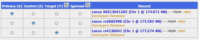
GN should generate a list of about 24 SNP markers. Pick the following three markers:
- Locus NES13041283 (the most proximal marker)
- Locus 11 on the list: rs3682996 (a central markers)
- Locus 24: rs4136041 (the most distal marker)
Add them to your collection. These markers bracket your region of interest and include one in the center. If you control for all three of them you are essentially killing any genetic variation that comes from Chr 1 at 176 Mb ±5 Mb. For a simple demonstration of partial correlation just use these three markers as your "Primary", "Control", and "Target" in a partial correlation test. The correlation will drop from r = 0.831 between the proximal and distal marker to a value of -0.041 if you control for the central marker. The screen shot below shows you how to replicate this simple test.
Simple Partial Correlation Setup for SNPs
Final ingredient: Add a set of some of the most interesting transcripts that are controlled by a QTL on Chr 1 between 174 and 178 (trans eQTLs) using fairly stringent search criteria in the Combined field.
At this point make sure you have switched back to the Hippocampus BXD RMA data set.
Here is the full search term that will find trans eQTLs that have LRS values higher than 18, AND the gene has to have expression above 9 units, AND the gene has to be associated with the Gene Ontology term "Translation" ID number 0006412.
LRS=(18 999 Chr1 174 179) transLRS=(18 999 10) mean=(9 20) GO:0006412
Select and add all 11 transcripts/probe sets/genes into the BXD Trait Collection. You can add other probe sets and genes to the list. The BXD collection now has about 48 transcripts and 2 SNPs in it.
Select all of these transcript traits and the two SNP markers and then initiate a partial correlation analysis. There is a button with a large arrow marked "Partial."
The steps for the Partial Correction involve:
- Set the two SNP markers as your CONTROL column variables.
- Select a single primary trait you will test. I used Fmn2, probe set 1450063_at.
- Select the target traits. I "IGNORED" all of the transcripts on Chr 1 other than my 11 target genes, none of which are on chromosome 1.
Making sense of the output table
The partial correlations between the primary trait and the targets shows you how much of the covariation between the two does NOT depend on the direct genetic effects of Fmn2. You expect the partial correlation to be lower because you have removed any genetic effects associated with Chr 1 (afterall you know that these 11 transcripts map to Chr 1 are have big trans eQTLs very close to Fmn2), but you are hoping that it is still significant. Have a look at this output page:
Partial Correlation Output
The partial correlation between Fmn2 and Nars changed dramatically, from the original "non-partial" value of r = 0.232 to the partial r = -0.414. That is an interesting change in polarity and magnitude. It means that the genetic effect located on Chr 1 that produces a positive correlation between these two transcripts strongly counteracts an otherwise negative correlation caused by other genetic effects NOT on distal Chr 1 and by other non-genetic factors. The partial correlations with Ei4g2, Mrpl42, and Yars also swings from positive to negative.
This seems quite interesting, but before we get too excited we should perform the same analysis with other "Primary" candidate genes near Fmn2 to see if this is an effect that is a specific effect. I fact, several other genes in the region have even more interesting differences between the standard "full" or zero-order correlation and the partial correlation.
Some probe sets clearly have nothing to do with our set of translation-related genes with QTLs that map to Chr 1. Pigm is an example of a gene that we can demote as a candidate based on the partial correlation results. But other genes, such as gremlin 2 (Grem2 get promoted, and may be even better candidates that Fmn2.
[RWW, July 17, 2010]
Back to Index
Last edit Jan 18, 2005, by KAG. Feb 19, by RWW. May 12, 2006 by RWW. Feb 15, 2012 by RWW
|